 Boost
C++ Libraries
...one of the most highly
regarded and expertly designed C++ library projects in the
world.
— Herb Sutter and Andrei
Alexandrescu, C++
Coding Standards
 Boost
C++ Libraries
...one of the most highly
regarded and expertly designed C++ library projects in the
world.
— Herb Sutter and Andrei
Alexandrescu, C++
Coding Standards
#include <boost/math/distributions/non_central_chi_squared.hpp>
namespace boost{ namespace math{

template <class RealType = double,
          class Policy   = policies::policy<> >
class non_central_chi_squared_distribution;

typedef non_central_chi_squared_distribution<> non_central_chi_squared;

template <class RealType, class Policy>
class non_central_chi_squared_distribution
{
public:
   typedef RealType  value_type;
   typedef Policy    policy_type;

   // Constructor:
   non_central_chi_squared_distribution(RealType v, RealType lambda);

   // Accessor to degrees of freedom parameter v:
   RealType degrees_of_freedom()const;

   // Accessor to non centrality parameter lambda:
   RealType non_centrality()const;

   // Parameter finders:
   static RealType find_degrees_of_freedom(RealType lambda, RealType x, RealType p);
   template <class A, class B, class C>
   static RealType find_degrees_of_freedom(const complemented3_type<A,B,C>& c);

   static RealType find_non_centrality(RealType v, RealType x, RealType p);
   template <class A, class B, class C>
   static RealType find_non_centrality(const complemented3_type<A,B,C>& c);
};

}} // namespaces
The noncentral chi-squared distribution is a generalization of the Chi Squared Distribution. If Xi are ν independent, normally distributed random variables with means μi and variances σi2, then the random variable

is distributed according to the noncentral chi-squared distribution.
The noncentral chi-squared distribution has two parameters: ν which specifies the number of degrees of freedom (i.e. the number of Xi), and λ which is related to the mean of the random variables Xi by:

(Note that some references define λ as one half of the above sum).
This leads to a PDF of:

where f(x;k) is the central chi-squared distribution PDF, and Iv(x) is a modified Bessel function of the first kind.
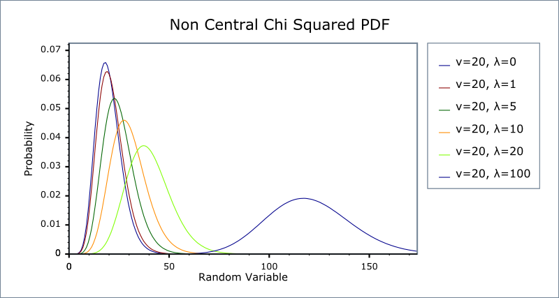
The following graph illustrates how the distribution changes for different values of λ:

non_central_chi_squared_distribution(RealType v, RealType lambda);
Constructs a Chi-Squared distribution with v degrees of freedom and non-centrality parameter lambda.
Requires v > 0 and lambda >= 0, otherwise calls domain_error.
RealType degrees_of_freedom()const;
Returns the parameter v from which this object was constructed.
RealType non_centrality()const;
Returns the parameter lambda from which this object was constructed.
static RealType find_degrees_of_freedom(RealType lambda, RealType x, RealType p);
This function returns the number of degrees of freedom v
such that: cdf(non_central_chi_squared<RealType,
Policy>(v, lambda),
x)
== p
template <class A, class B, class C> static RealType find_degrees_of_freedom(const complemented3_type<A,B,C>& c);
When called with argument boost::math::complement(lambda, x, q) this function returns the number of
degrees of freedom v such that:
cdf(complement(non_central_chi_squared<RealType,
Policy>(v, lambda),
x))
== q.
static RealType find_non_centrality(RealType v, RealType x, RealType p);
This function returns the non centrality parameter lambda such that:
cdf(non_central_chi_squared<RealType,
            Policy>(v, lambda),
            x)
            == p
template <class A, class B, class C> static RealType find_non_centrality(const complemented3_type<A,B,C>& c);
When called with argument boost::math::complement(v, x, q) this function returns the non centrality
parameter lambda such that:
cdf(complement(non_central_chi_squared<RealType,
            Policy>(v, lambda),
            x))
            == q
.
All the usual non-member accessor functions that are generic to all distributions are supported: Cumulative Distribution Function, Probability Density Function, Quantile, Hazard Function, Cumulative Hazard Function, mean, median, mode, variance, standard deviation, skewness, kurtosis, kurtosis_excess, range and support.
The domain of the random variable is [0, +∞].
There is a worked example for the noncentral chi-squared distribution.
The following table shows the peak errors (in units of epsilon) found on various platforms with various floating-point types, along with comparisons to the R-2.5.1 Math library. Unless otherwise specified, any floating-point type that is narrower than the one shown will have effectively zero error.
Table 17. Errors In CDF of the Noncentral Chi-Squared
|
Significand Size |
Platform and Compiler |
ν,λ < 200 |
ν,λ > 200 |
|---|---|---|---|
|
53 |
Win32, Visual C++ 8 |
Peak=50 Mean=9.9 R Peak=685 Mean=109 |
Peak=9780 Mean=718 R Peak=3x10⁸ Mean=2x10⁷ |
|
64 |
RedHat Linux IA32, gcc-4.1.1 |
Peak=270 Mean=27 |
Peak=7900 Mean=900 |
|
64 |
Redhat Linux IA64, gcc-3.4.4 |
Peak=107 Mean=17 |
Peak=5000 Mean=630 |
|
113 |
HPUX IA64, aCC A.06.06 |
Peak=270 Mean=20 |
Peak=4600 Mean=560 |
Error rates for the complement of the CDF and for the quantile functions
are broadly similar. Special mention should go to the mode
function: there is no closed form for this function, so it is evaluated
numerically by finding the maxima of the PDF: in principal this can not
produce an accuracy greater than the square root of the machine epsilon.
There are two sets of test data used to verify this implementation: firstly we can compare with published data, for example with Table 6 of "Self-Validating Computations of Probabilities for Selected Central and Noncentral Univariate Probability Functions", Morgan C. Wang and William J. Kennedy, Journal of the American Statistical Association, Vol. 89, No. 427. (Sep., 1994), pp. 878-887. Secondly, we have tables of test data, computed with this implementation and using interval arithmetic - this data should be accurate to at least 50 decimal digits - and is the used for our accuracy tests.
The CDF and its complement are evaluated as follows:
First we determine which of the two values (the CDF or its complement) is likely to be the smaller: for this we can use the relation due to Temme (see "Asymptotic and Numerical Aspects of the Noncentral Chi-Square Distribution", N. M. Temme, Computers Math. Applic. Vol 25, No. 5, 55-63, 1993) that:
F(ν,λ;ν+λ) ≈ 0.5
and so compute the CDF when the random variable is less than ν+λ, and its complement when the random variable is greater than ν+λ. If necessary the computed result is then subtracted from 1 to give the desired result (the CDF or its complement).
For small values of the non centrality parameter, the CDF is computed using the method of Ding (see "Algorithm AS 275: Computing the Non-Central #2 Distribution Function", Cherng G. Ding, Applied Statistics, Vol. 41, No. 2. (1992), pp. 478-482). This uses the following series representation:

which requires just one call to gamma_p_derivative with the subsequent terms being computed by recursion as shown above.
For larger values of the non-centrality parameter, Ding's method can take an unreasonable number of terms before convergence is achieved. Furthermore, the largest term is not the first term, so in extreme cases the first term may be zero, leading to a zero result, even though the true value may be non-zero.
Therefore, when the non-centrality parameter is greater than 200, the method due to Krishnamoorthy (see "Computing discrete mixtures of continuous distributions: noncentral chisquare, noncentral t and the distribution of the square of the sample multiple correlation coefficient", Denise Benton and K. Krishnamoorthy, Computational Statistics & Data Analysis, 43, (2003), 249-267) is used.
This method uses the well known sum:

Where Pa(x) is the incomplete gamma function.
The method starts at the λth term, which is where the Poisson weighting function achieves its maximum value, although this is not necessarily the largest overall term. Subsequent terms are calculated via the normal recurrence relations for the incomplete gamma function, and iteration proceeds both forwards and backwards until sufficient precision has been achieved. It should be noted that recurrence in the forwards direction of Pa(x) is numerically unstable. However, since we always start after the largest term in the series, numeric instability is introduced more slowly than the series converges.
Computation of the complement of the CDF uses an extension of Krishnamoorthy's method, given that:

we can again start at the λ'th term and proceed in both directions from there until the required precision is achieved. This time it is backwards recursion on the incomplete gamma function Qa(x) which is unstable. However, as long as we start well before the largest term, this is not an issue in practice.
The PDF is computed directly using the relation:

Where f(x; v) is the PDF of the central Chi Squared Distribution and Iv(x) is a modified Bessel function, see cyl_bessel_i. For small values of the non-centrality parameter the relation in terms of cyl_bessel_i is used. However, this method fails for large values of the non-centrality parameter, so in that case the infinite sum is evaluated using the method of Benton and Krishnamoorthy, and the usual recurrence relations for successive terms.
The quantile functions are computed by numeric inversion of the CDF.
There is no closed form for the mode of the noncentral chi-squared distribution: it is computed numerically by finding the maximum of the PDF. Likewise, the median is computed numerically via the quantile.
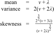
The remaining non-member functions use the following formulas:

Some analytic properties of noncentral distributions (particularly unimodality, and monotonicity of their modes) are surveyed and summarized by:
Andrea van Aubel & Wolfgang Gawronski, Applied Mathematics and Computation, 141 (2003) 3-12.